Project 4: Visibility on Terrains
- Assigned: Saturday, October 28
- Due: Wednesday November 8th
- Group policy: Partner-optional
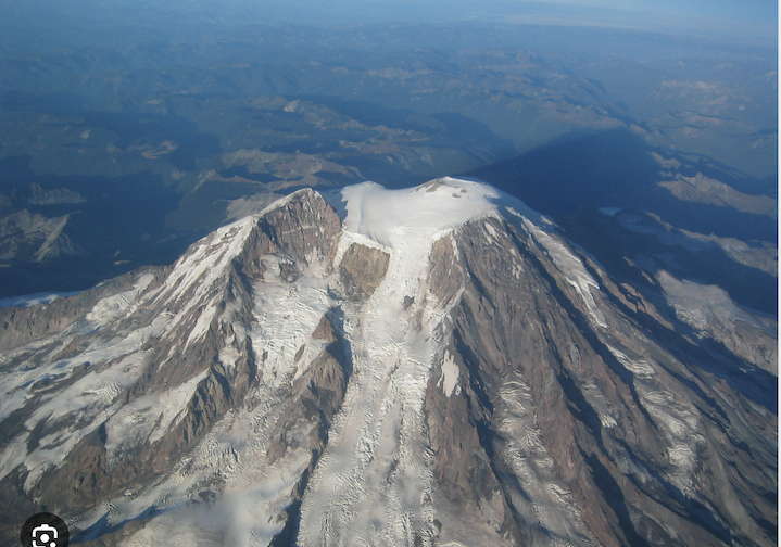
Have you ever wondered what would be the view from the top of Mt. Rainier at 14,410 ft? In this project you will (partially) answer this question, with several days of work and sweat over debugging, but without the strenous and difficult climb: You will write code to compute the viewshed of an arbitrary point on a terrain, download high resolution data for Mt. Rainier from OpenTopo, and use your code to compute viewsheds of points that fall approximately on the top.
Some interesting facts from NASA about Mt. Rainier.
Input: As input, your code will take the name of an elevation grid, the coordinates (r,c) of the viewpoint, the elevation of the viewpoint above the terrain, and the name of the viewshed grid to be created.
Output: Your code will compute the viewshed of the point (r,c) standing at the given elevation above ground level, and save it as an ascii grid in a file with the specified name. It will print the size of the viewshed (nb. of points that are visible). And it will create and save a bitmap of this viewshed, overlayed onto the elevation hillshade.
The interface
For example, running with
./vis -e ~/DEMs/rainier.asc -v vis.asc -r 1000 -c 1000 -h 10
or
./vis ~/DEMs/rainier.asc vis.asc 1000 1000 10
will compute the viewshed of point (r=1000, c=1000), standing 10 above ground level, and save the viewshed grid as vis.asc.
Datasets
To start you can use any of the datasets from previous projects.
Test datasets: You can download the datasets here
Eventually you will run your code on Mt. Rainier, which you can download directly from OpenTopography. I have downloaded a dataset which I’ll share with all of you so that we can compare results. It has ncols=26765 and nrows=24286, at below 1m resolution, for a total n = 650M points.


Algorithm
We talked about three different algorithms to compute the viewshed of a point:
- The straightforward algorithm
- The radial-sweep algorithm proposed by Van Kreveld.
- The algorithm that computes horizons in a concentric sweep
The radial sweep algorithm assumes cells have constant altitude/zenith throughout their span, which creates some artifacts in practice. So we are not going to use this algorithm.
The concentric sweep algorithm involves merging horizons which in turn involves computing intersection of segments on the horizon. This is tricky to write and get all special cases correct. Furthermore determining if a point is visible comes down to determining if a point is above or below a segment of the horizon, which is numerically unstable when points are very close to lines. So we are not going to use this algorithm either.
For this project you will implement the first algorithm: given a viewpoint v, traverse the grid and for each point p, determine if p is visible from v. As discussed in class, there are a couple of steps:
- find all the intersection points q between the horizonal projection of the segment vp and the grid lines
- for each such point q interpolate its height based on the grid segment it is on and compute the altitude of q with respect to v
- point p is visible if all the intersection points have the altitude below the altitude of p, and invisible otherwise.
Overview
The structure of the code is fairly simple. You will start by reading the command line arguments (and printing them).
(base) ltoma@XVR66RXWMT code % ./vis -e ~/DEMs/set1-30m.asc -r 100 -c 100 -v vis.asc
running with arguments:
	elev_name: /Users/ltoma/DEMs/set1-30m.asc
	vis_name: foo.asc
	vp=(100, 100, 0.0)
Then you will read the elevation gri, print some basic information about it (grid.c has a function to do this), and create a hillshade bitmap (note: my Mt. Rainier hillshade looked reversed, which is either because something is reverted in my code, or it is a visual effect. In any case, I generated a gradient colormap on the hillshade which looked better).
You will create and initialize a viewshed grid, compute the viewshed, create a bitmap overlayed on the hillshade of the terrain and save the viewshed grid to disk (grid.c has a function to do that). Finally you will free the memory for the grids and the pixel buffers.
compute_viewshed_grid(elev_grid, vis_grid, vr, vc, vh);
// create bitmap "map.vis-over-hillshade.bmp"
//save vis_grid to ascii file
//free grid
The computation of the viewshed grid is encapsulated in this function:
/*
 elev_grid: input elevation grid
 vis_grid: output viewshed grid, initialized to 0
 vr, vc, vh: viewpoint row, column, height
 populates vis_grid with values, a point is set to 1 if its visible from (vr,vc,vh)
*/
void compute_viewshed_grid(const Grid* elev_grid, Grid* vis_grid, int vr, int vc, int vh);
Note that its a good idea to initialize the viewshed grid as 0 (not visible), and update the points that are visible to 1. Viewsheds are usually (very) small, so it is more efficient to initialize all the grid as invisible and turn the visible points to 1 (visible), then the other way around.
const int VISIBLE = 1;
const int NOT_VISIBL = 0;
To determine what points are visible, compute_viewshed_grid will call another function:
/*
 elev_grid: input elevation grid
 r,c: row and column
 vr, vc, vh: viewpoint row, column, height
 returns 1 if point (r,c) is visible from (vr,vc,vh)
 returns 0 otherwise
*/
int is_point_visible(Grid* elev_grid, int r, int c, int vr, int vc, int vh);
This function is where you’ll spend most of your time.
Structure of your code
To work with grids and pixel buffers you will use the same files as before:
- stb_image_write.h
- pixel_buffer.h, pixel_buffer.c
- grid.h, grid.c
From the previous project you’ll use:
- map.h, map.c: Need to include grid.h and pixel_buffer.h. All functions to create bitmaps from grids are here.
If you want to create a separate function to visualize a viewshed grid, you will add it here.
You’ll create the following additional files:
vis.hpp, vis.cpp: Need to include grid.h. All the functions to compute the viewshed are here. The main functions that you need to implement are in the header, but you will need to add more helper functions.
vismain.c: The main() function is here. Read command line arguments from the user, create the viewshed grid,
and create the bitmaps. Includes grid.h, map.h, vis.hpp.
Once you accept the code on github classroom, a good place to start is writing your main() in vismain.c: read the command line arguments, read the elevation grid and create the hillshade map, create the viewshed grid and compute it. As you get things to compile, start with an empty compute_viewshed_grid()function, and then gradually add the code in, one small piece at a time.
You will spend most of your time writing the is_point_visible(..) function. Start by computing only the intersection with the horizontal grid lines; the viewshed you will see will be larger than the real one, because it is only filtering through half of the terrain. Once you add the intersections with the vertical segments (the other half), this will mark some of the points that were previously visible as invisible, so your viewshed will shrink to a smaller size.
Working with large data
A new piece in this project will be working with a large dataset. The Mt. Rainier dataset has a little over 650 million points and the ascii file mtrainier.asc uses 11GB of disk space. When you load it as a grid in memory, which stores elevation as a float, the elevation grid will occupy 4 x 650M = 2.6GB of memory. This is large! (Obviously, you do not want to test your code on this large dataset until it works smoothly on the smaller sets.)
The theoretical complexity of the viewshed algorithm is $O(n \sqrt n)$. This is evaluated as the total number of instructions executed by the algorithm assuming that:
- all data fits in memory
- all memory accesses take the same amount of time
- all instructions take the same amount of time.
Theoretical complexity is expressed using asymptotic notation, which hides all the constants in the running time. Algorithms that are in the same class of asymptotic complexity are considered equivalent. There are two reasons for doing this: First, counting instructions while assuming all instructions are equal means the constants are not accurate anyways. Second, by ignoring the constants the emphasis is placed on optimizing at the algorithmic level first, which should always be the first step.
In practice, these assumptions are not completely accurate and the running time will also depend on the type of instructions executed (some instructions are slower) and on the number and type of memory accesses.
Instructions are not all equal: When your code needs to work with large datasets, small variations in the number and type of instructions will have a large impact on the running time. One more expensive instruction, if executed 600 million times, will add significant extra time to your code. Be aware of the expensive instructions vs cheap instrictions. Multiplying or dividing by two, addition, increment — all these are instructions that run in a few clock cycles or machine instructions. Instructions like division and multiplications are more expensive. And library functions like computing trigonometric functions, arc tangents, and so one take 100 cycles or so. If we can avoid using these the code will get a big speed up.
Extra challenge: If you want to dig more into code optimization, check out using a profiler tool, which will give you exact statistics on how many times each function in the code is called and what percentage of the running time it makes up for. The rule of thumb is that you do not want to optimize a function that makes up for a small percentage of the total running time. You will want to focus your efforts on the function that has most impact on the running time.
Memory efficiency: Data is stored in a hirarchy of caches, and the difference in speed between accessing data in cache versus main memory versus extenal memory can be several orders of magnitude. Be aware of the memory footprint of your code (how much RAM it uses at any given time). The elevation grid and the viewshed grid will both have to be in memory, which will be around 5.2GB of RAM. If your code uses a hillshade grid, that’s 2.6GB more. In this case, plan it so that the hillshade and the viewshed grid do not exist at the same time, i.e. create the hillshade grid and the hillshade bitmap and then delete the hillshade grid, before you create the visibilty grid (not that the hillshade grid can be deleted once you copied it into the pixel buffer). In addition to the elevation and viewshed grids, you will also need two pixel buffers, which are also large.
So the main thing is to be aware of the main memory (RAM) footprint of your code especially as compared to the size of the main memory on your laptop. If for other project you did not worry about freeing memory, for this one you will want to delete a grid and a buffer as soon as you don’t need them. If the memory footprint is larger than the available RAM, the system will place the data onto external memory, which will be 2-3 orders of magnitude slower to access than main memory.
Fastest code award
There will be prizes for the fastest code! Stay tuned for details.
The Report
You will write a report showcasing your work including:
- The dataset(s) you used, location, number of rows and columns, resolution and provenance.
- Results.
- Run your code with set1.asc vp=(250,250), h=0, 10, 50, 100.
- Run your code on southport.asc, vp=(1000,1000)
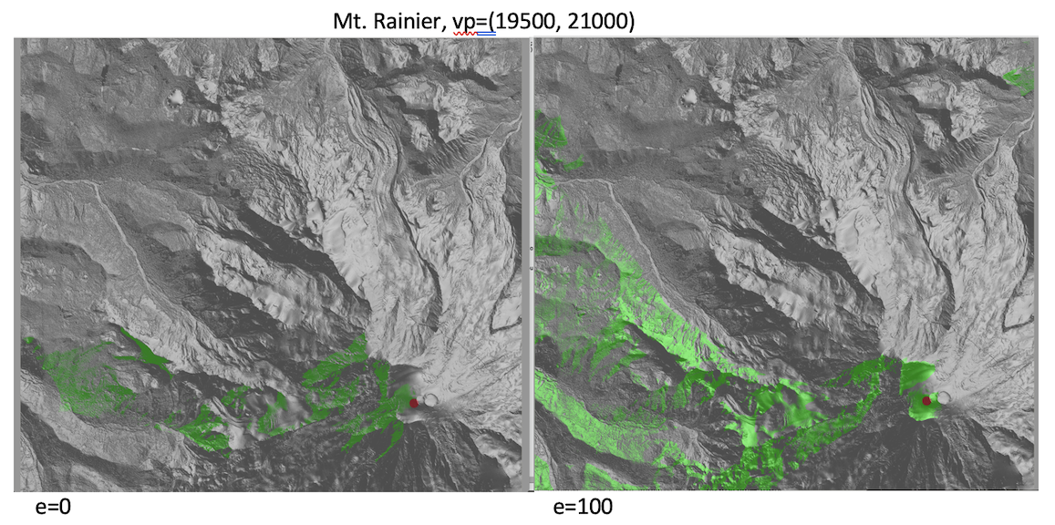
- Run your code on MtRainier on one of the viewpoints in the figure below
- Run your code on YOUR_DATASET.asc on a well chosen viewpoint.
- Maps. For each dataset create viewshed-over-hillshade bitmap. Note that if the bitmaps are large you should NOT add them to the repository (github won’t let you anyways).
- Bugs and extra features.
- Effort. Time you spent in: thinking, Programming; Testing; documenting; total.
- Reflection. Prompts: how challenging did you find this project? what did you learn by doing this project? What did you wish you did differently? If you worked as a team, how did that go? What would you like to explore further? — you don’t need to address all.
What to turn in
- Check in your code to the github repository
- Message me the report.
Final remarks
As always, starting early and making progress every day is important so that your learning is rewarding and enjoyable. Coding projects become overwhelming if put off too long. Think one piece at a time, and remember this is an opportunity to learn.
A 3000-level class means you work towards being independent and debugging your code independently. Use the internet as much as you can, to answer your questions on how to do things in C/C++, syntax and so on. Write code incrementally, in small pieces at a time, so that you always know where the error is coming from. Use the bitmaps and prints to know what you are computing at all times.
Put differently, if you don’t start early, you likely won’t be able to finish, and if you don’t approach coding incrementally, you likely won’t be able to debug your code.
Enjoy!
Results

set1 viewshed size:
Set1 vp=(250, 250)
h=0:   viewshed size=11978
h=10:  viewshed size=14486
h=50:  viewshed size=25327
h=200: viewshed size=52570
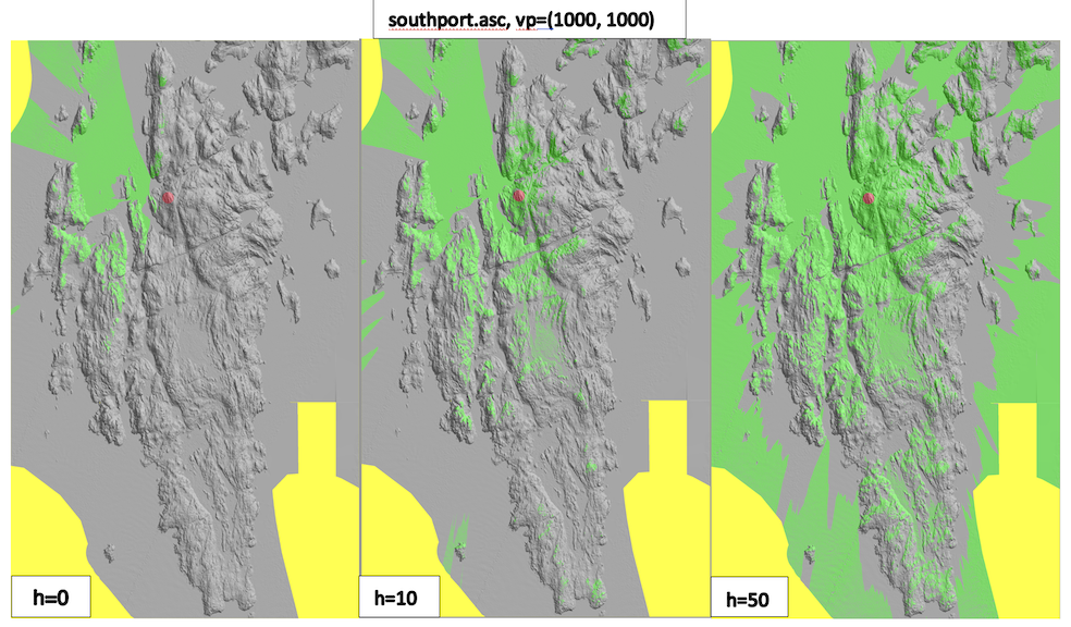
Southport viewshed sizes:
southport vp=(1000, 1000)
e=0:  viewshed size=555941
e=10: viewshed size=1059023
e=50: viewshed size=3669179
For Mt. Rainier, it turns out it is not easy to find a spot on the rim of the crater with good visibility of the surroundings. Inside the crater all you can see is the crater. Outside the crater there are deep valleys and rims which obstruct the view.
Finding a point at the foothills of the mountain with good visibility of the top crater is not straightforward either —- I tried a few points but none had a good view of the crater.
Below are some of the attempts. Reading the elevation grid in memory takes about 180 seconds (on my computer); computing the viewshed takes 50-60 seconds, but that is using the faster, horizon-based algorithm; your code will be slower.